What is xG? – 2

The xG metric gives the probability of a shot resulting in a goal.

This probability is calculated from several characteristics of the shot, such as the position of the ball on the pitch, the shooting angle, the number of nearby opponents, the type of assist received, the body part used to shoot, among others.

It does not take into account who took the shot.

The term stands for “expected goals”. If we add up the xG of all of a team’s shots in a match, we get an estimate of how many goals that team should have scored.

If a team had a total xG of 1.5 in a match, we can’t tell whether it had a few clear-cut chances or many low-quality ones.

A widely used measure of chance quality is the match xG divided by the number of shots. This gives us an idea of how good, on average, the chances a team created were.

Let’s look at an example using the 2022 men’s World Cup. The code below gets the StatsBomb event data.

library(kickoff)
library(dplyr)

# Get SB open competitions
sb_competitions <- kickoff::sb_open_competitions()

# Get 2022 World Cup
wc_2022 <- sb_competitions |>
  filter(
    competition_name == "FIFA World Cup",
    competition_gender == "male",
    season_name == 2022
  )

# Get 2022 World Cup matches
wc_2022_matches <- kickoff::sb_open_matches(wc_2022)

# Get 2022 World Cup events
wc_2022_events <- kickoff::sb_open_events(wc_2022_matches)

StatsBomb has its own xG model. We can access the xG of each shot through the shot.statsbomb_xg column.

final_match <- wc_2022_matches |>
  filter(competition_stage.name == "Final")

final_match_xg <- wc_2022_events |>
  filter(match_id == final_match$match_id) |>
  # Remove penalty shootouts
  filter(period %in% 1:4) |>
  group_by(team.name) |>
  summarise(match_xg = sum(shot.statsbomb_xg, na.rm = TRUE))

In the final, Argentina had a total xG of 2.76, while France’s was 2.27. Note that we only consider regular time and extra time, excluding the penalty shootout.

Both teams scored more goals than their xG would suggest (the match ended 3–3).

This is no accident!

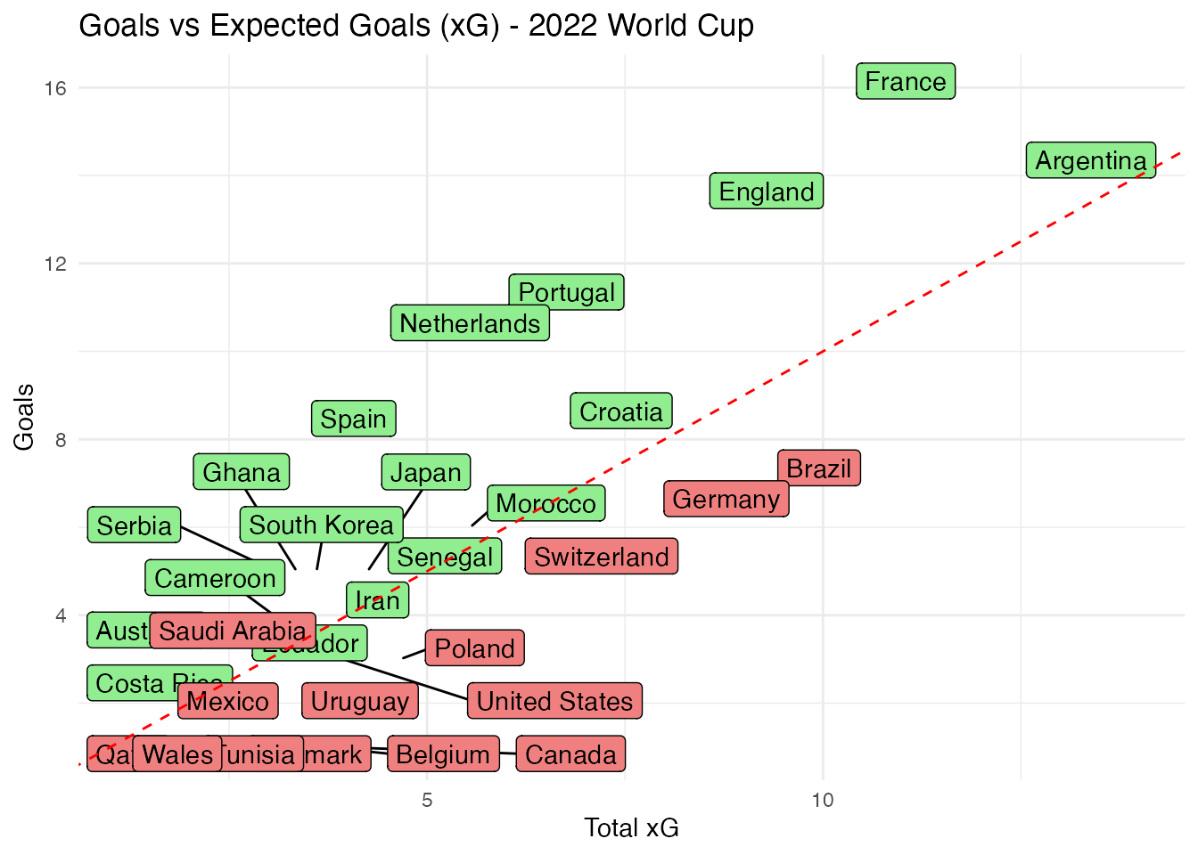
Since the xG of a shot is a probability calculated from a historical average of similar shots, good teams are expected to outperform their xG.

The chart below shows each team’s xG over the whole tournament versus the number of goals scored (excluding own goals). Teams in green, above the dashed line, scored more goals than their xG would suggest, while teams in red scored fewer.

library(ggplot2)

wc_2022_goals_vs_xg <- wc_2022_events |>
  filter(period %in% 1:4) |>
  group_by(team.name) |>
  summarise(
    total_xg = sum(shot.statsbomb_xg, na.rm = TRUE),
    goals = sum(shot.outcome.name == "Goal", na.rm = TRUE)
  ) |>
  arrange(desc(goals))

wc_2022_goals_vs_xg |>
  mutate(
    fill = ifelse(goals > total_xg, "lightgreen", "lightcoral")
  ) |>
  ggplot(aes(x = total_xg, y = goals, label = team.name, fill = I(fill))) +
  ggrepel::geom_label_repel(max.overlaps = 30) +
  geom_abline(slope = 1, intercept = 0, linetype = "dashed", color = "red") +
  labs(
    title = "Goals vs Expected Goals (xG) - 2022 World Cup",
    x = "Total xG",
    y = "Goals"
  ) +
  theme_minimal()